Bayesian Neural Network
Published:

Bayesian Neural Network
In contrast to traditional neural networks, the weight of Bayesian Neural Networks(BNN) is allocated a probability distribution rather than a single value or point estimate. BNN has the following advantages:
- Ensemble Model. Because the weights in the Bayesian neural network are allocated a probability distribution, then multiple sampling of BNN on a certain weight distribution can be integrated for prediction, which is equivalent to ensemble.
- Uncertainty of the prediction. Multiple sampling on a distribution would help us get the standard deviation of the prediction, which tells us the uncertainty of the prediction.
- Regularization.
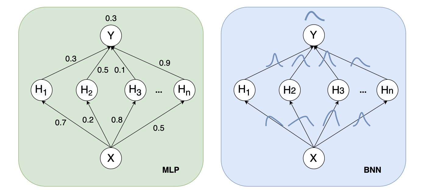
Instead of learning the weights directly, a Bayesian neural network is trained using variational inference to learn the parameters of these distributions(μ and σ when the weights are allocated a Gaussian Distribution):

Figure 1.1: Left: the weights are fixed during forward propagation. Right: each weight is assigned a distribution.
A neural network can be considered as a probabilistic model $p(y \vert x,w)$. y is referred to a set of classes while a categorical distribution is referred to as $p(y \vert x,w)$. y is a continuous variable in regression, while $p(y \vert x,w)$ is a Gaussian distribution.
Given a training dataset D{$x^{(i)}$, $y^{(i)}$}. For a neural network, we could construct the likelihood function $p(D \vert \textbf{w}) = \prod_{i} p(y^{i} \vert \textbf{x}^{i}, \textbf{w})$. which is a function of parameters $\textbf{w}$. Maximizing the likelihood function gives the Maximimum Likelihood Estimate (MLE) of $\textbf{w}$. The usual optimization objective during training is the negative log likelihood. For a categorical distribution this is the cross entropy error function, for a Gaussian distribution this is proportional to the sum of squares error function. MLE can lead to severe overfitting though.
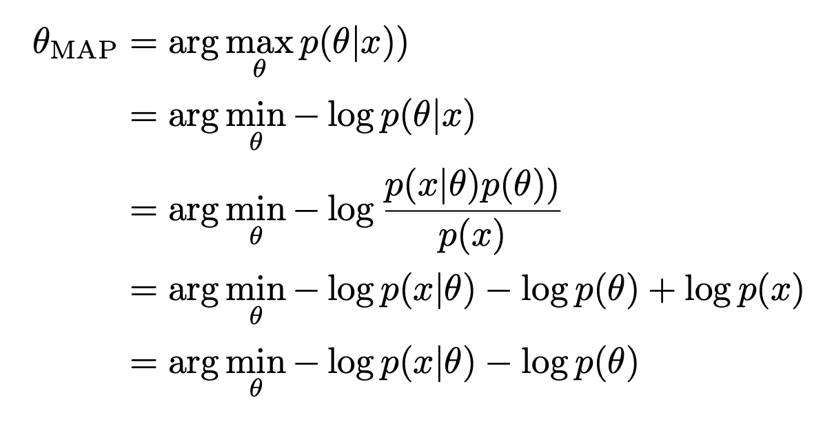
\[\begin{aligned} \theta_{MLE} = & \underset{\theta}{\operatorname{argmax}} log\ p(D \vert w) \\ = & \underset{\theta}{\operatorname{argmax}} \sum_{i=1}^{n} log \ p((y_{i} \vert x_{i} , w) \end{aligned}\]In bayesian’s view, we could add a prior $p(w)$ to the MLE, which became Maximum a posteriori estimation(MAP) :
\[\begin{aligned} \theta_{MAP} = & \underset{\theta}{\operatorname{argmax}}log \ p(w \vert D) \\ = & \underset{\theta}{\operatorname{argmax}} log \ p(D \vert w) + log\ p(w) - log\ p(D) \\ = & \underset{\theta}{\operatorname{argmax}} log \ p(D \vert w) + log\ p(w) \end{aligned}\]Which $log\ p(w)$ is equivalent to an L2 regularization term (which tends to be a small value). And when the prior is a Laplace Distribution, $log\ p(w)$ is equivalent to an L1 regularization (tends to be 0 to make the weights sparse).
Both MLE and MAP give point estimates of parameters. If we instead had a full posterior distribution over parameters we could make predictions that take weight uncertainty into account. Then the probabilistic model would be:
\[\begin{aligned} p(y \vert x) = &E_{p(w \vert D)}[p(y \vert x,w)] \\ = & \int_{w}^{} p(y \vert x, w)p(w \vert D)dw \end{aligned}\]While there are two problems:
[1] Unfortunately, an analytical solution for the posterior $p(w \vert D)$ in neural networks is untractable :
It is equivalent to summing (or integrating) all possible w, so the input data distribution $p(D)$ is untractable.
[2] $p(y\vert x)$ is also not easy to find, because it is equivalent to computing the prediction of the neural network for every possible $p(w\vert D)$
We therefore have to approximate the true posterior with a variational distribution $q(w\vert \theta )$ of known functional form whose parameters we want to estimate. This can be done by minimizing the Kullback-Leibler divergence between $q(w\vert \theta )$and the true posterior $q(w\vert D )$.
\[\begin{aligned} \theta^{(t+1)} =& \underset{\theta}{\operatorname{argmin}}KL[q(w\vert \theta )\vert \vert p(w\vert D)] \\ =& \underset{\theta}{\operatorname{argmin}} \sum_{w} q(w \vert \theta) log(\frac{q(w\vert \theta)}{p(w\vert D)}) \\ =& \underset{\theta}{\operatorname{argmin}} \sum_{w} q(w \vert \theta) log(\frac{q(w\vert \theta) p(D)}{p(D\vert w) p(w)}) \\ =& \underset{\theta}{\operatorname{argmin}} \sum_{w} q(w \vert \theta) log(\frac{q(w\vert \theta)}{p(w)}) -\sum_{w} q(w\vert \theta)log(p(D\vert w) + \sum_{w}q(w\vert \theta)p(D) \\ =& \underset{\theta}{\operatorname{argmin}} KL[q(w\vert \theta)\vert \vert p(s)] - \mathbb{E}_{q(w\vert \theta)}[p(D\vert w)]\\ \end{aligned}\]The corresponding optimization objective or cost function is
\[\mathcal{F(D, \theta)} = \underset{complexity \ cost}{KL[q(w\vert \theta)\vert \vert p(w)]} - \underset{likelihood cost}{\mathbb{E}_{q(w\vert \theta)}[p(D\vert w)]}\]This is known as the variational free energy. The first term is the Kullback-Leibler divergence between the variational distribution $q(w\vert θ)$ and the prior $p(w)$ and is called the complexity cost. The second term is the expected value of the likelihood w.r.t. the variational distribution and is called the likelihood cost. By re-arranging the KL term, the cost function can also be written as
\[\mathcal{F(D, \theta)} = \mathbb{E}_{q(w\vert \theta)}[q(w\vert \theta)] - \mathbb{E}_{q{w\vert \theta}}[p(w)] - \mathbb{E}_{q(w\vert \theta)}[p(D\vert w)]\]To be continued.


