Maximum Likelihood Estimation and Bayesian Estimation

Maximum Likelihood Estimation

The frequentists view is that the data is a repeatable random sample (random variable) with a specific frequency/probability. The underlying parameters and probabilities remain constant during this repeatable process and that the variation is due to variability in $X_{n}$ and not the probability distribution (which is fixed for a certain event/process).

Eg: Define $P(X)$ is the probability density function(PDF) of $X$ with parameter θ. After we got a sequence of observation (X₁, X₂, …, X_n) = (x₁, x₂, …, x_n), we would like to get the estimate for parameter θ.

In frequentists view, $\theta$ has specific value. Event (X₁, X₂, …, X_n) = (x₁, x₂, …, x_n) is most likely to occur when $\theta = \theta_{MLE}$, which $\theta_{MLE}$ is the Maximum Likelihood Estimation of $\theta$.

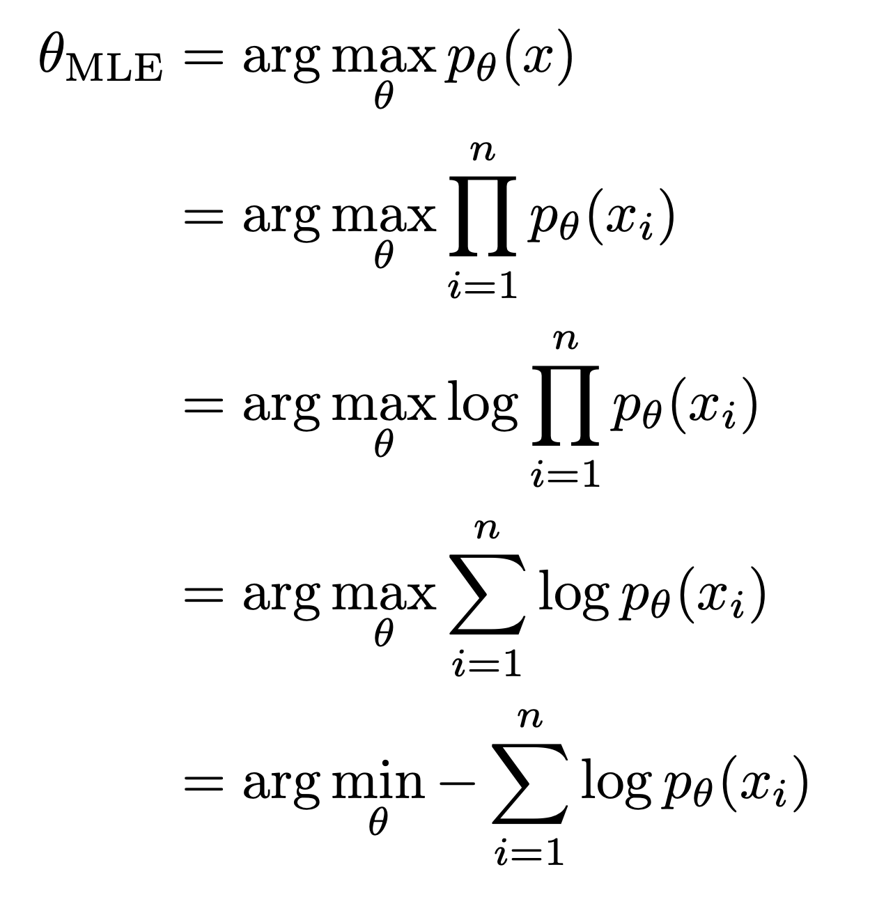
The item that needs to be optimized is Negative Log Likelihood (NLL).

Bayesian Estimation

The bayesian view is that the data is fixed while the frequency/probability for a certain event can change, which means the parameters of the distribution changes. In effect, the data that you get changes the prior distribution of a parameter which gets updated for each set of data. (the prior is changed when using different dataset)

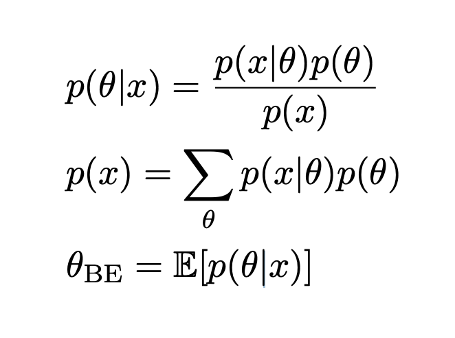
$p(\theta)$: prior, which is the probability distribution that would express one’s beliefs about this quantity before some evidence is taken into account.
$p(x \vert\theta)$: likelihood, what would x be when θ is known.
$p(\theta|x)$: posterior, the distribution of the parameter.
$p(x)$: prior of the dataset, a constant that is independent of the parameter θ to be estimated.

Bayesian estimation is equivalent to that \theta obeys the prior distribution $p(\theta)$, and then corrects the prior distribution according to the observed samples, and finally obtains the posterior distribution $p(\theta\vert x)$, and then takes the posterior distribution Expected as an estimate of the parameter.

Bayesian estimation equals to MLE when $p(\theta)$ is Gaussian distribution.

Maximum a posteriori estimation

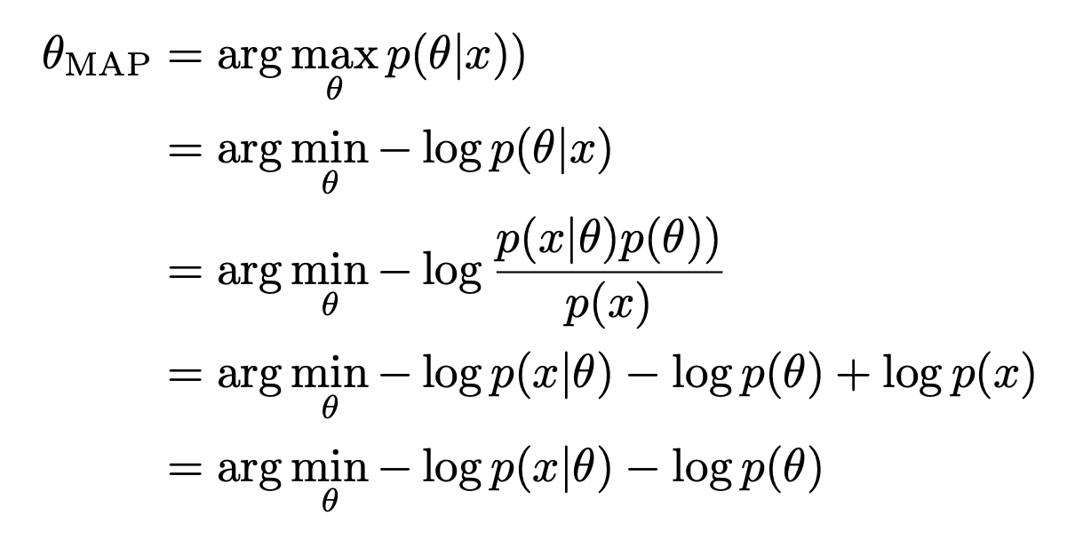
We can calculate the posterior distribution of $\theta$ using Bayes’ theorem. A maximum a posteriori probability (MAP) estimate is an estimate of an unknown quantity, that equals the mode of the posterior distribution.

The $-log\ p(x \vert\theta)$ is Negative Log Likelihood(NLL). Therefore, compared with MLE, MAP is an additional a priori term $p(\theta)$ during optimization. In some cases, $-log\ p(\theta)$ can be used as a regularizer in structured risk when using MLE, such as when the prior is a Gaussian distribution:

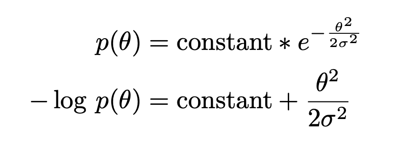
At this time, $-log\ p(\theta)$ is equivalent to an L2 regularization term (which tends to be a small value).

And when the prior is a Laplace Distribution, $-log\ p(\theta)$ is equivalent to an L1 regularization (tends to be 0 to make the weights sparse).

MAP provides an intuitive way to design complex but interpretable regularization terms, for example more complex regularization terms can be obtained by taking mixture Gaussian distributions as priors.

Comparison

If we toss a coin 10 times, and get 7 heads and 3 tails. MAE would tell the probability of heads is 0.7. While if MAP takes a prior of head as 0.5, the final result would be 0.5-0.7.