RBF, SVM and MLP for Classification

RBF, SVM and MLP for Classification

Abstract

A report of the experiment on Radial Basis Function(RBF), Self-organizing map(SOM), Support vector machine(SVM) and a two-fully connected layer network(MLP) with back-propagation.

Setup on which the code was tested

- python==3.7
- numpy==1.19.2

I. Data Analysis

Before the experiment, it is important to analyze the dataset first. The dataset contains 330 training samples, 21 testing samples, each sample is a vector with length of 33. There are two classes. Label of the data is [-1 , 1].

Samples labeled as 1 accounted for approximately 65% of the total, samples labeled as -1 accounted for approximately 35%. Among the 33 features, the value is mostly close to one of 1.0, 0.0 and -1.0.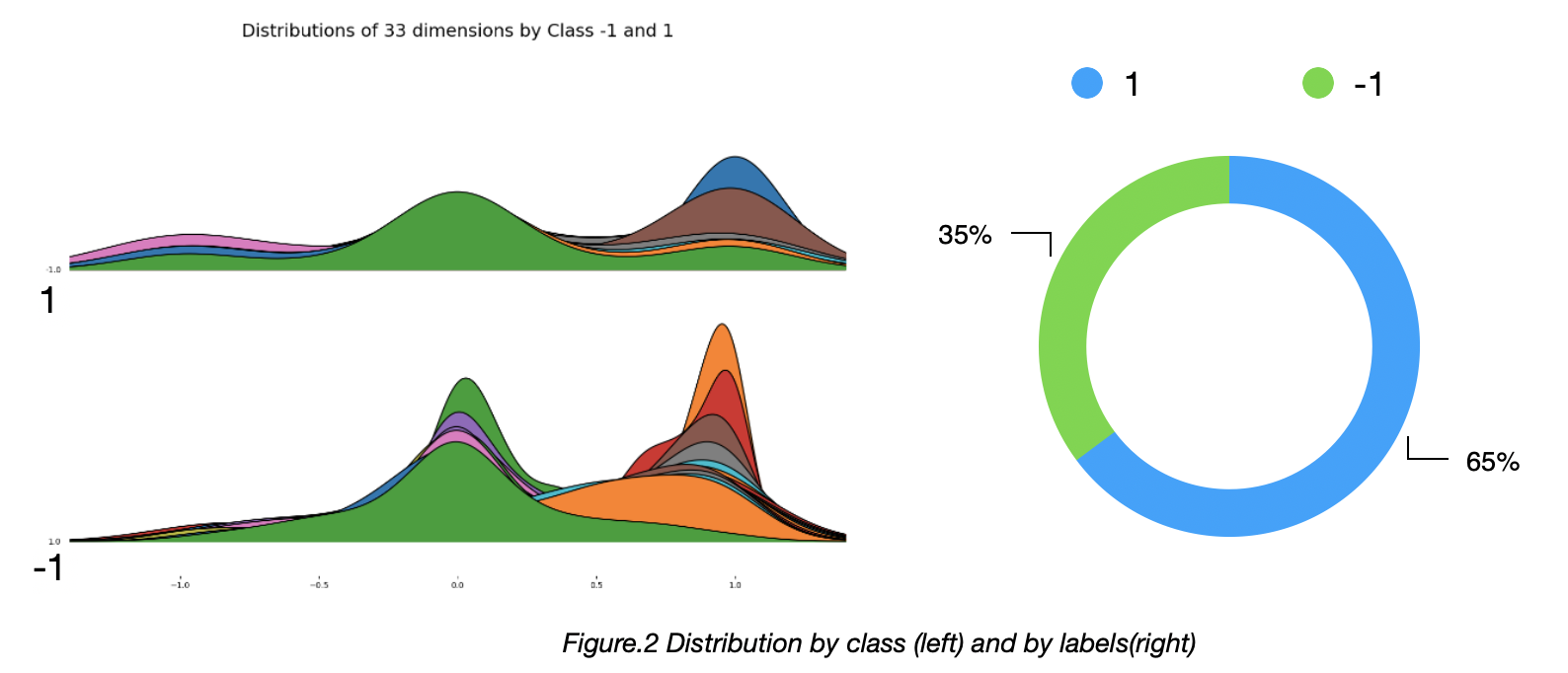

II. Radial Basis Function

Structure

Number of the neurons is first set to 10. The centers(neurons) are generated by k-means.

center_num = 10
model = KMeans(n_clusters=center_num, max_iter=1500)
model.fit(data_train)
centers = model.cluster_centers_

Results

The output of the RBF is shown in the figure , so next we need to pick a threshold for the classification. 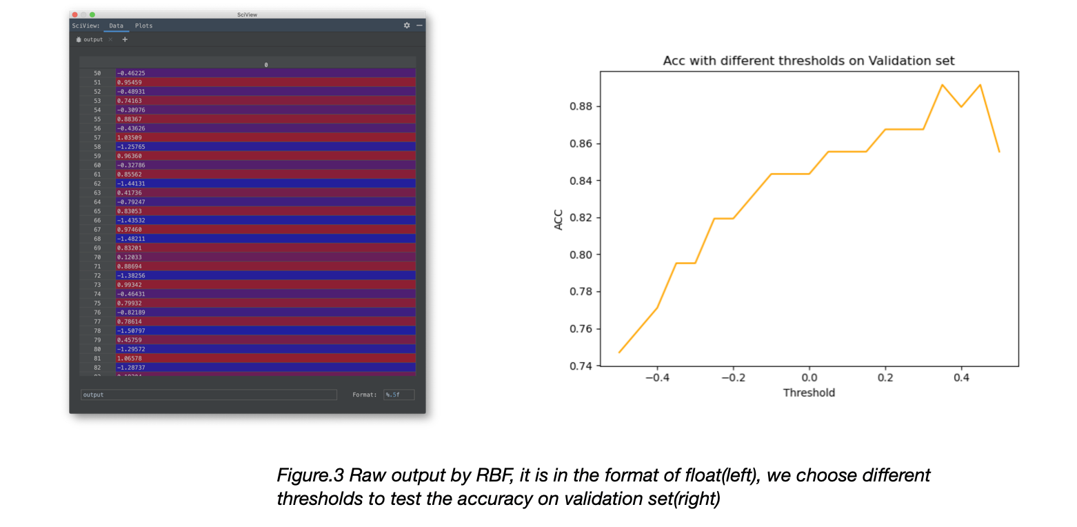We choose threshold from [-0.5, 0.5], step set as 0.05, to test how different thresholds influence the Accuracy. We set threshold as 0.20, and test the model with 21 testing data, the output is shown in Figure.3.

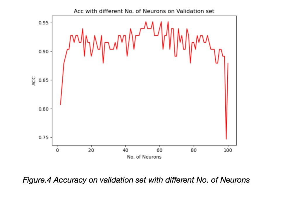
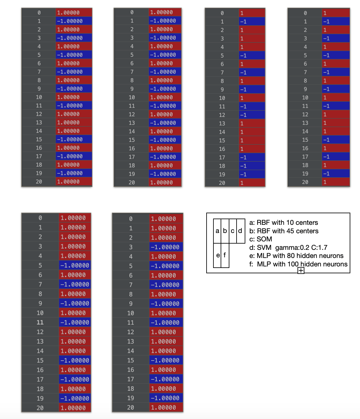
To test how the number of neurons influence the performance, we choose it from [5, 100] and the accuracy is shown in the Figure.4. We set the number of neurons to be 45; threshold as 0.3 and test the model with 21 testing data, the output is shown in the appendix A.

III. Self-organizing map

We use k-means and SOM to generate the centers for RBF network.

Structure

num_neural: 81
num_iteration: 500 * num_neural = 40,500
sigma: 3, (at the iteration t we have sigma(t) = sigma / (1 + t/T), where T = num_iteration/2
learning_rate: 0.5, (at the iteration t we have learning_rate(t) = learning_rate / (1 + t/T) )
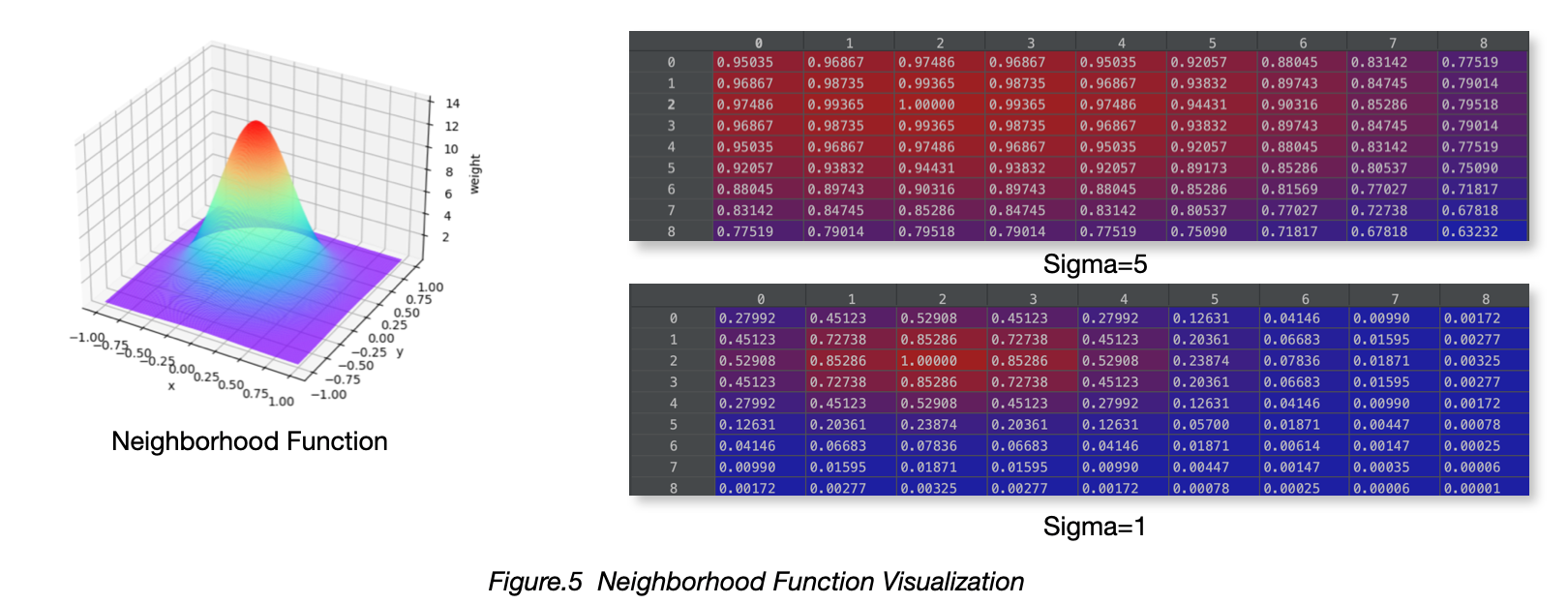
Neighborhood Function: Gaussian distribution with sigma=1 and sigma=5
Weight initializing: Picking random samples from data.

Results

Visualizing Data

To visualize the result of the training we plot the distance map using a pseudo color where the neurons of the maps are displayed as an array of cells and the color represents the (weights) distance from the neighbor neurons. On top of the pseudo color we add markers that represent the samples mapped in the specific cells:

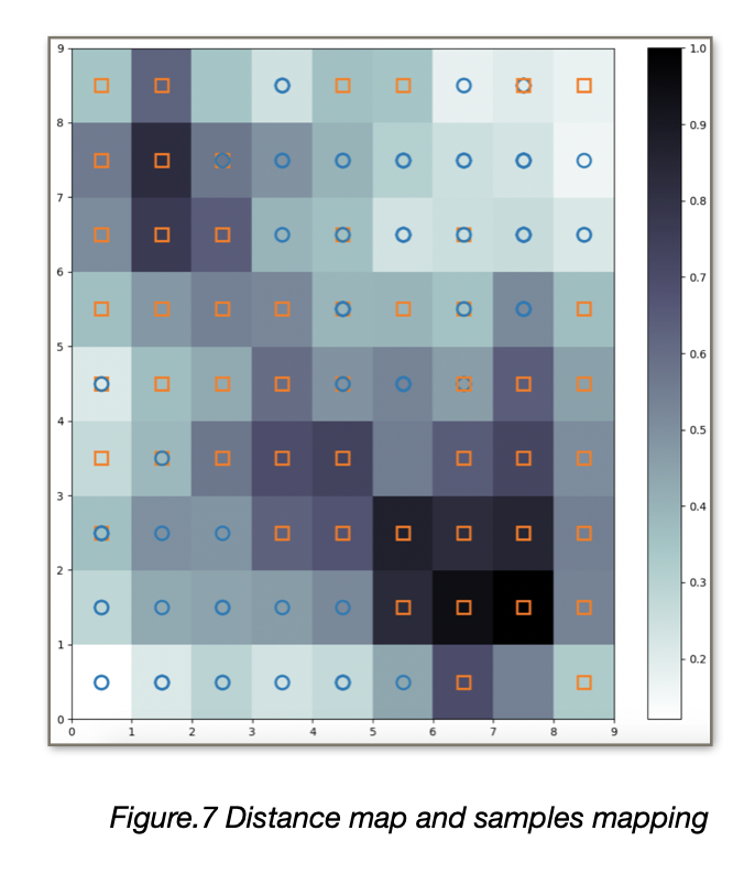
To have an overview of how the samples are distributed across the map a scatter chart can be used where each dot represents the coordinates of the winning neuron. A random offset is added to avoid overlaps between points within the same cell.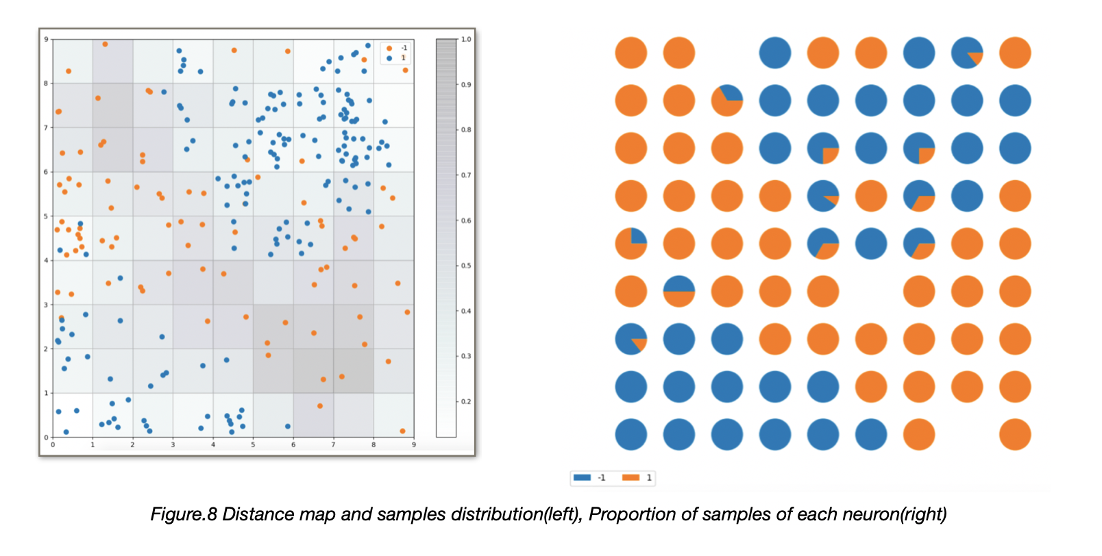

Because this is a supervised problem, we can visualize the proportion of samples per class falling in a specific neuron using a pie chart per neuron is shown in the Figure.8. For testing data, we could calculate the distance with the neurons and select the neuron that is most similar with the data, then we could do the classification with the SOM.

IV. Support vector machine

Structure

C = 1.0 Kernel: Radial basis function kernel Gamma = 0.1

Results

Acc of the training set = 96.26%. Acc of the testing set = 94.50%.

We also run a sequence experiment to test how the different C is influence the performance of the SVM. A Bigger C would cause model to be overfitting, shown in the Figure.9.

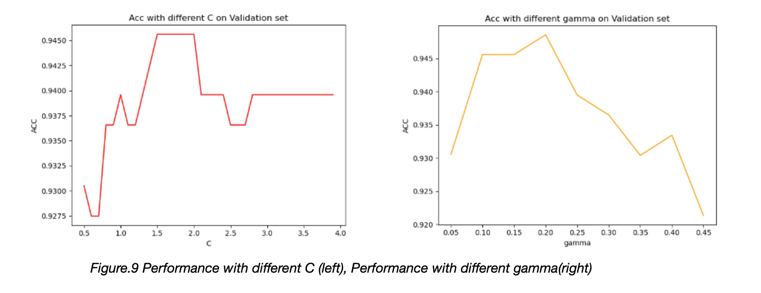
Gamma in the RBF kernel is also a hyper-param to be tuned, a model with bigger gamma will have fewer support vectors.

V. Multilayer Perceptron

Structure

Loss: MSE
Optimizer: SGD
Dropout rate: 0.5

Results

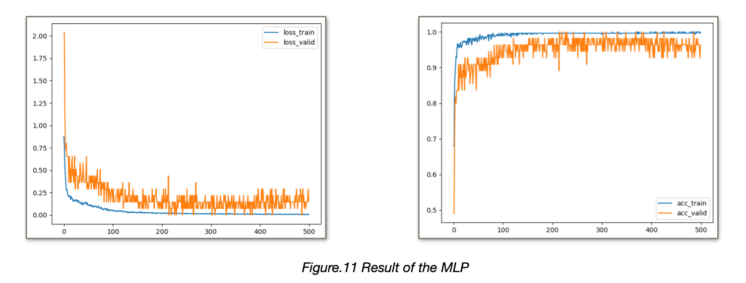
We ran for 30,000 epochs in total, and results are shown in Figure.11.

For different no. of neurons, we test the performance of the MLP, results shown in Figure.12.

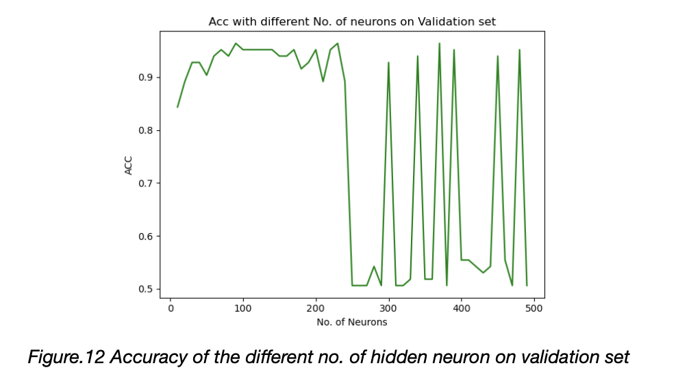
We find out that the network has more parameters would cause unstable and overfitting. And 330 samples is not enough for deep learning. In this task, traditional neural network beats the MLP.

VI. Conclusion

1.RBF needs pre-train to find the proper centers, there are many methods that could find the centers: Random picking/Top-down/Bottom-up/K-means/SOM/Gradient Descent.

2.SVM is fast, The SVM learning problem can be expressed as a convex optimization problem, so known effective algorithms can be used to find the global minimum of the objective function. Other classification methods (such as rule-based classifiers and artificial neural networks) use a strategy based on greedy learning to search the hypothesis space. This method generally only obtains a local optimal solution.

3.SOM can be used for classification by doing: for each neural we store the label of the classes that appeared most frequently in the training process.

4.MLP with too many parameters would cause unstable performance, in this case, for stability, RBF and SVM is better than MLP.

Appendix

Issues

The above is the description of all the work for the algorithms. If you encounter unclear or controversial issues, feel free to contact Leslie Wong.